Heavy, parameterized, or poorly designed CDS views often cause SAP Analytics Cloud (SAC) dashboards to run slowly or fail altogether. For developers and solution architects, understanding how to build lean, high-performance CDS views is critical. By carefully designing these views, you can ensure they work efficiently in both SAC Live (real-time) and SAC Import (load) models. Using core tools like ADT and RSRT, you can proactively test, optimize, and validate your CDS views. The key takeaway is simple: most SAC performance problems originate in CDS design, not in SAC itself.
Why This Matters
Executives and business users care about fast dashboards, reliable reporting, and low system load. A well-designed CDS view directly reduces latency, simplifies SAC models, and avoids expensive redesign cycles. Think of CDS as the foundation: if it’s unstable, SAC cannot deliver a smooth user experience.
Understanding SAC Live vs Import
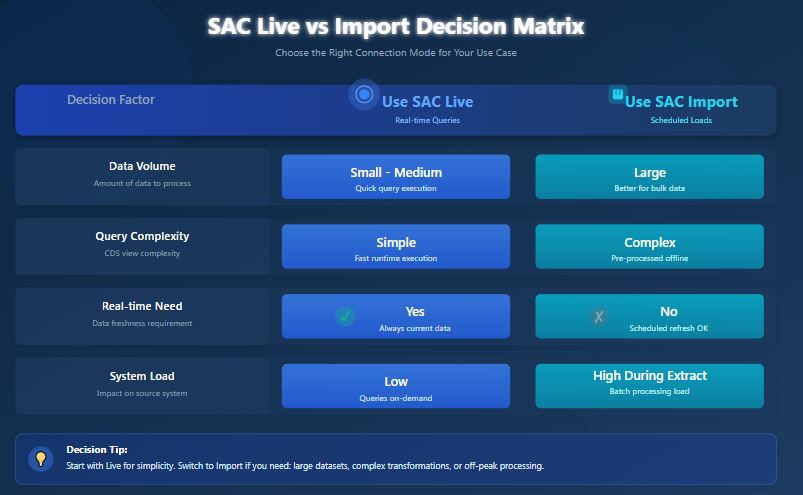
SAC works in two modes, each with different CDS requirements:
- Live Mode: Queries execute directly on HANA at runtime. Performance depends entirely on CDS efficiency.
- Import (Load) Mode: Data is extracted into SAC and stored. CDS must provide stable, parameter-free datasets for scheduled loads.
Warning: If a view runs slowly in RSRT, it will run slowly in SAC Live. Always test in RSRT first.
CDS Layering: Keep It Clean
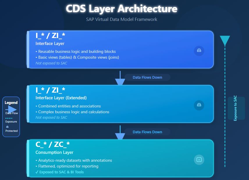
A layered CDS architecture improves reusability, clarity, and performance. SAP’s Virtual Data Model (VDM) provides a standardized framework for organizing CDS views into distinct layers.
Understanding the Layers
| Interface Layer (I_* / ZI_*) | Consumption Layer (C_* / ZC_*) | |
|---|---|---|
| Purpose | Reusable building blocks and business logic | Analytics-ready datasets optimized for reporting |
| Contains | • Basic views (on tables) • Composite views (joins) • Foundation laye | • Flattened structures • Analytics annotations • Denormalized data |
| Characteristics | • Reusable logic for multiple views • Both basic and composite views • Should NOT be exposed to SAC | • ONLY layer exposed to SAC • Optimized for analytics • Single exposure point |
| Naming | • I_* = SAP standard • ZI_* = Custom (Z = customer namespace) Standard CDS annotations | • C_* = SAP standard • ZC_* = Custom (Z = customer namespace) |
| Annotations | Standard CDS annotations | @Analytics.dataCategory • #CUBE (facts) • #DIMENSION (master data) |
| Exposed to SAC? | NO | YES |
Naming Convention Summary
- I_* = SAP standard interface view
- ZI_* = Custom interface view (Z = customer namespace)
- C_* = SAP standard consumption view
- ZC_* = Custom consumption view (Z = customer namespace)
Best Practice
Always separate reusable business logic (interface layer) from analytics-optimized views (consumption layer). This separation allows you to:
- Reuse common logic across multiple consumption views
- Optimize each layer for its specific purpose
- Maintain and test views independently
- Clearly communicate which views are intended for end-user consumption
Warning: Exposing I_* or ZI_* views directly to SAC violates the VDM architecture and can lead to performance issues, maintenance complexity, and unpredictable behavior.
Common CDS Mistakes That Hurt SAC
Many SAC projects fail not because of SAC itself, but due to over-engineered CDS. Examples include:
- Exposing I_* views directly to SAC
- Deep join chains across multiple tables
- Excessive runtime calculations in top-level views
- Wide datasets with unused columns
- Parameterized views for import models
Each of these mistakes can create slow dashboards, high memory usage, and unpredictable results.
Principles for Lean CDS Design
To make CDS views lean:
- Push Logic Down Early: Perform calculations in lower layers to reduce runtime overhead.
- Keep Views Narrow: Only expose fields required for analytics. Extra columns increase processing time.
- Minimize Joins: Flatten complex join chains and pre-aggregate where possible.
- Separate Reuse and Consumption: I_* for reusable building blocks, C_* or ZC_* for SAC exposure.
- Avoid Parameters for Import: Replace them with filters or derived fields to create stable datasets.
- Test in RSRT: If it runs slowly in RSRT, it will run slowly in SAC.
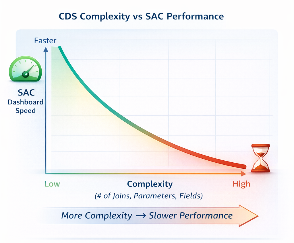
SAC Live queries execute in real time on HANA, which means:
- Dashboard speed depends entirely on CDS performance
- Poor joins or calculations immediately slow queries
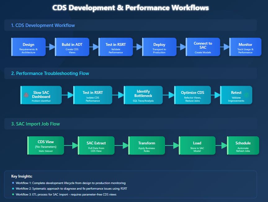
- RSRT is your primary debugging tool
- Always test consumption CDS views in RSRT before exposing them to SAC Live
SAC Import extracts and stores data. The rules:
- No mandatory parameters: SAC cannot supply them during import
- Stable, predictable datasets: Required for scheduled loads
- Use consumption CDS only: Avoid exposing lower-level views
- Pre-resolve logic: Replace dynamic calculations or parameters with derived fields
Warning: A parameterized CDS view might work perfectly in RSRT but will fail in SAC Import if you don’t create a static consumption version.
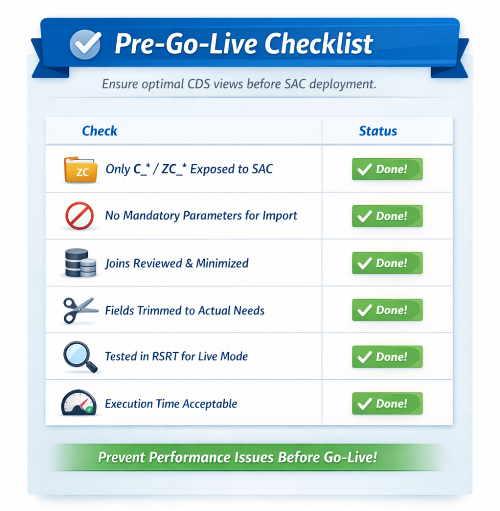
This simple checklist prevents most SAC performance issues before users even see them.
Conclusion
Building high-performing SAC dashboards starts long before anything reaches SAP Analytics Cloud.
- ADT helps you design and validate CDS views,
- RSRT allows you to test and debug query execution, and
- SQL Analyzer or ST05 lets you trace database performance issues – but the real success factor is lean, well-structured CDS architecture.
Fast SAC experiences come from proper modeling that reduces system load, accelerates delivery, and builds business confidence in analytics. Optimizing CDS isn’t about micro-tuning every join or column; it’s about simplicity, predictability, and sound design. When done right, SAC Live feels instantaneous, Import jobs run reliably, and users trust their data foundation. For deeper insight into VDM principles, SAP’s official documentation provides additional guidance
For more details on VDM architecture, see SAP’s official VDM documentation.
Next, we will review the foundational CDS layering principles – I_, C_, and 2C_ – that support all SAP Embedded Analytics designs.