To stay ahead, businesses need to understand not only where they are but also where they’re heading. With SAP Analytics Cloud Smart Predict, forecasting future trends becomes effortless through intuitive Time Series Models – no coding or data science expertise required.
In this post, we’ll explore how time series forecasting works in SAC, how to build and interpret models, and how to transform predictive insights into better business outcomes.
What Is a Time Series Model?
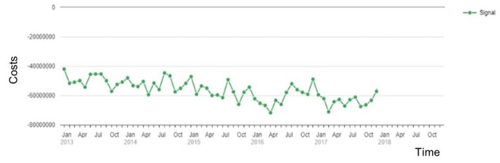
A time series is a collection of data points recorded at regular intervals – such as daily sales, monthly revenue, or quarterly expenses. Time series forecasting uses these historical values to predict future outcomes. For example:
- How will next month’s revenue evolve?
- What stock levels will we need next week?
- How might cash flow fluctuate next quarter?
These insights help organizations plan more effectively and respond proactively to trends.
Data Requirements: Building a Strong Foundation
To build a time series model in SAC Smart Predict, your dataset must contain:
- A target variable (signal): the metric you want to forecast, like sales or revenue.
- A date variable: timestamps for each data point, formatted properly (e.g., YYYY-MM-DD).
- Optional influencer variables: factors that may impact the signal, such as marketing campaigns, holidays, or weather.
These influencers help refine predictions and capture real-world effects on your business outcomes
Understanding Variable Roles
To build an effective time series model, it is crucial to understand the role of each variable in your dataset:
Signal Variable
- The main variable you want to forecast or explain. Example: If you want to predict product sales for the next six months, product sales is your signal variable.
Date Variable
- The variable representing the time dimension is mandatory for all time series models.
- SAC requires specific date formats to interpret the data correctly. See the supported formats and examples below:
| Description | Date Format Examples |
|---|---|
| Supported SAC Formats | YYYY-MM-DD YYYY/MM/DD YYYY/MM-DD YYYY-MM/DD YYYYMMDD YYYY-MM-DD hh:mm:ss |
| Example: January 25, 2018 | 2018-01-25 2018/01/25 2018/01-25 2018-01/25 20180125 |
Ensuring that your signal and date variables are correctly defined and formatted is the first step toward accurate forecasting in SAC Smart Predict
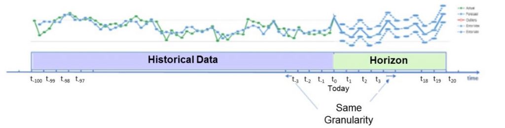
Setting the Forecast Horizon
Your forecast horizon defines how far into the future the model predicts. A general rule of thumb: use a 5:1 ratio of historical to forecast data. For instance, with 100 months of past data, SAC can reliably predict 20 future values. The further the horizon, the more uncertainty exists – so balancing depth of history with forecast length is essential.
How SAC Smart Predict Builds the Model
When you train a time series model:
- SAC sorts the data chronologically and splits it into two parts: 75% for training , 25% for validation
- SAC then tests multiple model candidates, combining techniques like: Auto-Regression (AR): Predicting future values using past fluctuations. Exponential Smoothing: Adjusting forecasts dynamically to account for trends and seasonality.
- The model with the best performance, lowest error, and appropriate complexity is selected automatically.
This process ensures your model is both accurate and interpretable.
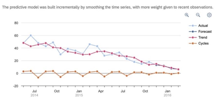
Understanding Key Components of Time Series
Every time series can be broken down into 4 components:
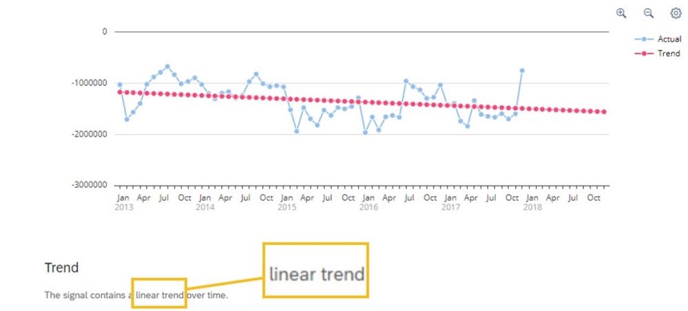
- Trend – The long-term direction of your data (increasing or decreasing). Trend can be linear or non-linear. It could be the result of influences such as population growth, price inflation and general economic changes.
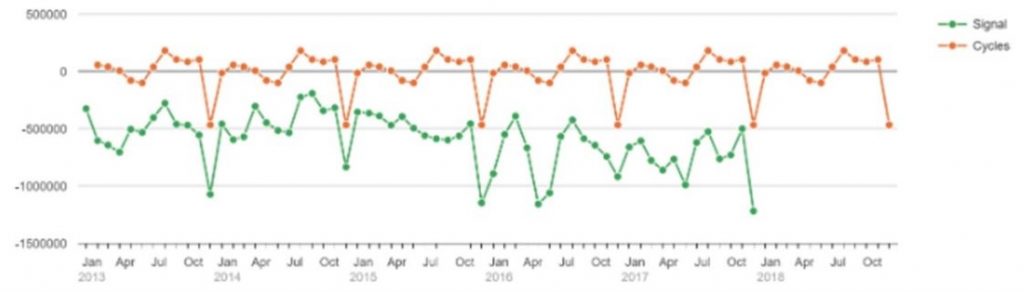
- Seasonality & Cycles – Repetitive patterns linked to time (like monthly peaks or yearly dips).
- Fluctuations – Short-term variations or noise around the trend.
- Residuals – Random effects that can’t be explained by other components
SAC automatically detects these elements to explain how your data behaves – and why.
Detecting the Cycles in SAC
SAP Analytics Cloud automatically searches for two types of cycles when building a time series model:
- Periodicity – Natural events that repeat at fixed intervals, called a period.
- Seasonality – Calendar-based patterns such as:
- dayOfWeek
- dayOfMonth
- dayOfYear
- weekOfYear
- monthOfYear
- hourOfDay
These cycles are also evaluated for potential influencer variables, helping the model understand recurring effects across time dimensions. All of these cycles are automatically detected and tested within Smart Predict.
Note: To accurately detect cycles – especially those with long periods or strong seasonality – it’s essential to include enough historical data in your dataset.
Exponential Smoothing: Stabilizing and Refining Forecasts
Exponential Smoothing is one of the key forecasting techniques integrated into SAC Smart Predict. It smooths out random fluctuations to make forecasts more stable and realistic.
During training, SAC tests multiple models:
- Double Exponential Smoothing – best for data with trends but no strong seasonality.
- Triple Exponential Smoothing – ideal when both trend and seasonality exist.
The model that achieves the highest accuracy automatically becomes part of the winning predictive model. This approach ensures that forecasts:
- Adapt even when cycles vary in strength or timing.
- Handle multiple seasonalities effectively.
- Remain automated, transparent, and reliable for business use.
Incorporating Influencer Variables
Adding influencer variables can significantly improve your forecast accuracy. Examples include:
- Marketing campaign dates
- Product launch timelines
- Weather data
- Month-end or quarter-end effects
These variables must have known future values to remain relevant within your forecast horizon.
Evaluating Model Accuracy: Horizon-Wide MAPE
SAC Smart Predict measures forecast quality using the Horizon-Wide mean Absolute Percentage Error (MAPE) – a metric that expresses prediction error as a percentage.
- A lower MAPE means a more accurate model.
- A MAPE of 0% indicates a perfect forecast.
This gives analysts a clear, scale-independent way to compare multiple predictive models.
Dealing with Outliers and Anomalies
Not all data points follow the expected trend. SAC automatically identifies outliers – unusual values that deviate significantly from typical behavior. These anomalies could result from data entry errors, unexpected events, or rare market fluctuations. By detecting outliers, SAC ensures they do not distort the model, maintaining forecast accuracy.
Additionally, analysts can visualize these outliers on Forecast vs. Actual charts, helping to pinpoint specific events or errors that need further investigation. In some cases, outliers may reveal valuable insights about unusual customer behavior, seasonal spikes, or operational issues, allowing businesses to make data-driven adjustments rather than ignoring irregularities.
Segmented Time Series Models
Sometimes, trends differ across regions, stores, or products.
A useful feature of SAC is segmented time series modeling, which automatically creates distinct models for each segment (up to 1,000). This means you can forecast:
- Sales by store
- Demand by region
- Energy use by sector
This approach maintains consistent predictive logic, performance metrics, and accuracy across every group. Segmented modeling ensures that local variations are captured, providing more granular and actionable insights for each segment of your business.
Training and Forecasting in SAC
Creating a time series model in SAC is straightforward:
- Navigate to Predictive Scenarios → Time Series Forecast.
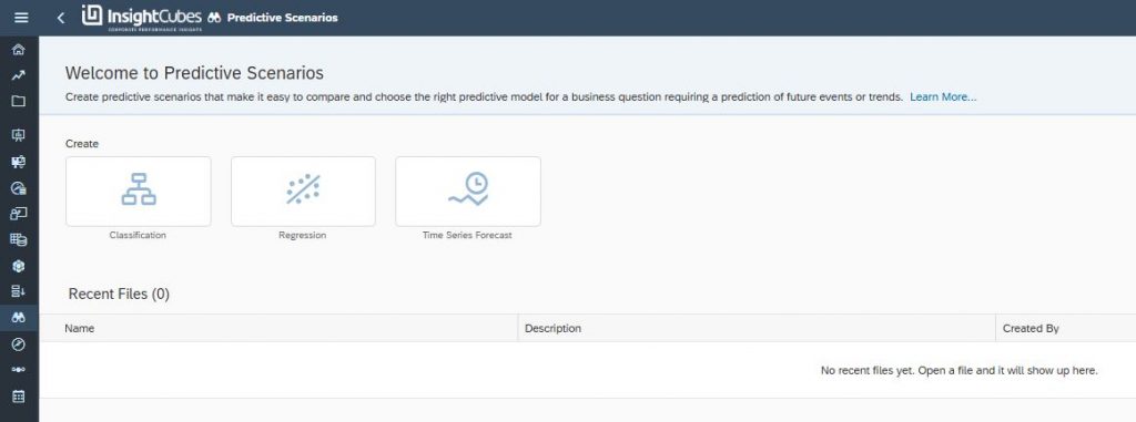
- Select your data source and signal variable.
- Define your date variable and forecast horizon.
- Optionally, specify entities and influencers.
- Click Train to let Smart Predict build and test multiple models automatically.
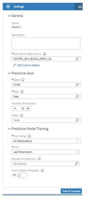
Predictive Model Training Options: The Train Using field allows you to control how historical data is used to build the model:
- All Observations – Uses the full dataset for training.
- Window of Observations – Restricts training to a specific period (e.g., last 3 months, 2 years).
You can also define:
- Until / Last Observation – Uses the most recent data as the cutoff.
- Until / User-Defined Date – Uses a specific date in the dataset as the cutoff.
- Exclude as Influencer – Removes selected variables from influencing the forecast.
- Force Positive Forecasts – Converts any negative forecasts to zero if they are not relevant for your business scenario.
Once trained, you can review performance indicators, adjust settings, and retrain for optimization.
Technical Limitations of Time Series Models
While SAP Analytics Cloud Smart Predict is powerful, there are some technical limits to keep in mind:
- Maximum columns: Your input dataset must not exceed 1,000 columns, as the model generates additional columns during application. Exceeding this limit may block the process.
- Segmented models: For segmented forecasts, it is recommended to have a maximum of 120 forecasts per segment and up to 1,000 segments.
- Data refresh: Acquired datasets cannot be refreshed; you must upload a new dataset and retrain the model to update predictions.
- Live datasets: Changes in live SAP HANA tables appear immediately in SAC, but updating the predictive model still requires retraining.
By keeping these limitations in mind, analysts can plan their data structure and model configuration efficiently, avoiding errors during forecasting.
Analyzing and Applying the Results
After training, SAC provides visual and tabular outputs, including:
- Forecast vs. Actual charts
- Signal Decomposition (Trend, Cycle, Fluctuation)
- Lagged Predictor Contributions showing how past data influences the future
You can then apply the model to create an output dataset that stores your forecasts, complete with confidence intervals and performance indicators.
Predict the Future with Confidence
SAP Analytics Cloud Smart Predict brings automated time series forecasting into the hands of business users.
From detecting trends and seasonality to managing segmented forecasts and influencers, SAC simplifies predictive modeling – making it both accessible and actionable. By mastering time series models, organizations can move beyond descriptive analytics and start anticipating what’s next with data-driven foresight.
In the next blog, we will explore how Regression Model in SAP Analytics Cloud can help you identify key drivers and transform data into actionable business insights.